In this article I’m gonna talk about normal unpacking for unsigned 8 bit per channel normal maps. If you are a bit familiar with this topic, you may know the usual formula[a] :
$$Normal=Unpack(Map)=2 \cdot Map-1$$But there’s another formula you probably have seen:
$$Normal=Unpack(Map)=\frac{(Map\cdot255-128)}{127}$$The second formula is used to get rid of the quantization error in zero. I will discuss in detail below the difference between these two equations and what they mean in term of quantization errors.
TL;DR
The (1) formula has a low quantization error and a perturbation of 0.3 degrees for neutral normals. With (2) the error on neutral normals is zero but the general quantization error increases. It is impossible to get rid of the quantization error, it can only be moved; thus there is no best function. You can see in the last section a live example of these two formulas applied to a normal map. There is no visible difference between the twos.
Normal Packing
Normal mapping is a technique used in computer graphics to enhance the level of detail of surfaces with a relatively[b] small number of polygons. Surface normals are usually stored as RGB images where the X, Y, Z components of the normal vectors are stored in the RGB channels. As said above, here I’m focusing on unsigned 8 bit per channel RGB images. This means that each image channel can contain 256 integer values from 0 to 255. During the packing process each normal vector’s coordinate is converted into an integer value in the range [0, 255]. Being a normal vector a unit vector of length 1, its coordinates are real numbers in the range [-1, 1]. So the packing algorithm must remap a real number from [-1, 1] into an integer in [0, 255]. Since at shader level the RGB components of a normal map are normalized in [0, 1], let’s get rid of this 255 by including a division by 255 in the packing algorithm. So our final mapping is from the continuous [-1, 1] range to the discontinuous [0, 1] range made of 255 levels. We can split the packing task into two steps:
- Remap coordinates from [-1, 1] to [0, 1]
- Quantize each coordinate into 256 levels
Here is the formula for the first step where N is the normal vector:
$$Remap(N)=\frac{N+1}{2}$$
And here is the second step:
$$Pack(N)=Quantize_{256}(Remap(N))=Quantize_{256}\left(\frac{N+1}{2}\right)$$
Before going on, let’s have a closer look at the quantization process in the next section.
Quantization
Quantization is the process of mapping a large set of input values to a (countable) smaller set. Here we want to define a \(Quantize_{m}\) function to put in the (4) formula above. We want a function that takes as input a value in [0, 1] and outputs one of the m quantized values in the same range. Let’s try with this function:
$$Quantize^{floor}_{m+1}= \frac{\left\lfloor x \cdot m \right\rfloor}{m} = \frac{floor(x \cdot m)}{m}$$
Note the \(m+1\) I have put above. If we cut a segment in \(m\) equal parts, we get \(m+1\) points: one point for each part plus a closure point on the last part (see image below). So if we want \(m+1\) levels of quantization, we have to divide by \(m\).

In the (5) function above, we are multiplying \(x\) times \(m\) and then taking the integer part of the result with the floor function (represented with the \(\lfloor\rfloor\) or \(floor()\) notation); we are also dividing by \(m\) to rescale the result back to [0, 1]. Here is a graph showing this function for \(m=5\):

Note the quantization error in the image above. The largest quantization error is \(\frac{1}{m}\), 0.2 for \(m=5\). We can do better than this if we take the nearest integer instead of the largest previous integer returned by the floor function. So let’s use the round function:
$$Quantize^{round}_{m+1}=\frac{round(x \cdot m)}{m}=\frac{\left\lfloor x \cdot m + \frac{1}{2}\right\rfloor}{m}$$

Note how we halved the max error value using the round function. Now the largest quantization error is (in absolute value) \(\frac{1}{2m}\), equal to 0.1 for \(m = 5\).
We can compute the mean error by measuring the area between the two functions in the graphs.
$$MeanError=\frac{1}{b-a}\cdot\int_{a}^{b}x-Quantize_{m}(x)\text{d}x$$
For the QuantizeFloor function we have to add up the area of m right triangles with base and height equal to \(\frac{1}{m}\). Each area is \(\frac{1}{m}\cdot\frac{1}{m}\cdot\frac{1}{2}=\frac{1}{2m^2}\) and the total area is:
$$MeanError_{floor}=\frac{1}{2m^2}\cdot m=\frac{1}{2m}$$
In the case of the QuantizeRound function is pretty clear from the graph that the sum of the positive errors and negative errors is zero:
$$MeanError_{round}=0$$
A mean error equal to zero tells us that positive and negative errors are symmetrical, but doesn’t tell anything about the error variance which is how much the error is spread outside of the mean value. To get this information we can compute the Mean Squared Error which incorporates the variance and the bias of the quantization error.
$$MSE=\frac{1}{b-a}\cdot\int_{a}^{b}\left(x-Quantize_{m}(x)\right)^2\text{d}x$$
For the QuantizeFloor we can compute the integral on the first triangle on the left and then multiply the result by m. If we look at the graph, we see that the error function is \(x\), so the squared error is \(x^2\), and being the interval size equal to \(\frac{1}{m}\) we have:
$$MSE_{floor}=m\cdot\int_{0}^{\frac{1}{m}}x^2\text{d}x=m\cdot\left[\frac{1}{3m^3}-0\right]=\frac{1}{3m^2}$$
The above value takes into account both the bias, which in the floor quantization is \(\frac{1}{2m}\), and the variance.
If we consider the QuantizeRound, we can compute the integral on the first triangle (which is smaller than the previous one) and than we have to multiply the result times \(2m\) which is the number of little triangles in the round quantization.
$$MSE_{round}=2m\cdot\int_{0}^{\frac{1}{2m}}x^2\text{d}x=2m\cdot\left[\frac{1}{3\cdot8\cdot m^3}-0\right]=\frac{1}{12m^2}$$
If we want to reduce the quantization error, we want a small bias and a small variance, hence we have to minimize the MSE. As seen above, the best quantization function is the round quantization. This is the function used by a modelling tool when we bake a normal map, and we will use this function in the next sections.
Normal Unpacking
Now let’s apply the quantization function found in the last section to the packing formula:
$$Pack(N)=Quantize_{256}\left(\frac{N+1}{2}\right)=\frac{Round\left(\frac{N+1}{2}\cdot255\right)}{255}$$
The above function outputs normalized values in [0, 1], the same values we get in shader when we sample a normal map texture.
Now let’s define the unpacking function. The simplest function is just a remapping from [0, 1] to [-1, 1]:
$$Unpack_{a}(Map)=2 \cdot Map-1$$
To analyze the unpacking function we define a compound function by applying the unpack after the pack function:
$$N_{a}(x)=Unpack_{a}(Pack(x))=2 \cdot \frac{Round\left(\frac{N+1}{2}\cdot255\right)}{255} – 1$$
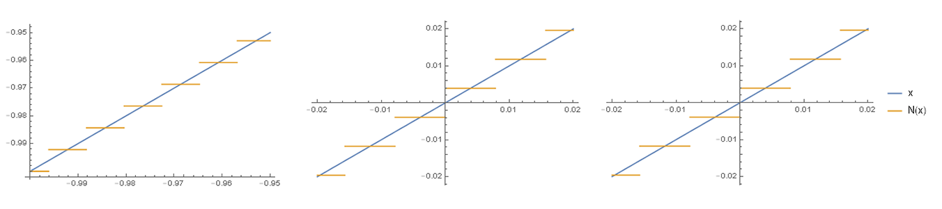
Has we can see in the image above, the quantization error is causing an error in zero. Let’s compute the value of \(N(x)\) on these three points: -1, 0, 1:
$$N_{a}(-1)=-1 \space , \space \space N_{a}(0)=\frac{1}{255} \space , \space \space N_{a}(1)=1$$
We have zero error in -1 and 1. The error in 0 is due to the fact that the input value zero is mapped to 127.5 and rounded to 128. Is this really a problem?
If we were using this packing algorithm to store an analog control value, the X or Y value of an analog stick for example, the error in zero could be a problem. A bias in zero should be filtered for the same reason we set a dead zone to filter hardware biases on analog controllers.
In the case of a Normal vector, the bias in zero will cause an error on neutral normals, which are up unit vectors: \([0, 0, 1]\). After the quantization, neutral normals will be unpacked to \(\left[\frac{1}{255}, \frac{1}{255}, 1 \right]\). This error will perturb the normal which will be rotated by an angle of:
$$NormalPerturbation=Arctan\left(\frac{\sqrt{2}}{255}\right)=0.317^{\circ}$$
Now, if we want to get rid of the error in zero while maintaining a linear unpacking function, we have two options: we can translate the unpacking down by \(\frac{1}{255}\), but this will introduce an error in 1 and -1. The other option is to enforce two equations: \(N(0)=0\) and \(N(1)=1\). Let’s define a new unpacking function. The first step is enforcing \(N(0)=0\). We said that 0 is mapped to 128. So we can start by subtracting 128 from the input remapped in [0, 255].
$$Unpack_{b}(x)=x \cdot 255 – 128$$
Let’s see the values on \(N_{b}\) in 0 and 1:
$$N_{b}(0)=Unpack_{b}(Pack(0))=0$$
$$N_{b}(1)=Unpack_{b}(Pack(1))=127$$
Now we enforce \(N_{b}(1)=1\), so we divide by 127:
$$Unpack_{b}(x)=\frac{x \cdot 255 – 128}{127}$$
Let’s plot again the compound function:
$$N_{b}(x)=Unpack_{b}(Pack(x))=\frac{Round\left(\frac{N+1}{2}\cdot255\right) – 128}{127}$$
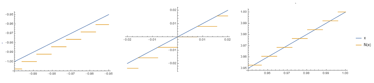
As you can see above, we have removed the error in zero and the value in 1 is also correct, but we have increased the quantization error for the negative values. The greatest error is in -1 where N is:
$$N_{b}(-1)= – \frac{128}{127}=-1 – \frac{1}{127}$$
We can think that to obtain \(N_{b}(x)\) we have done an anticlockwise rotation of the graph of \(N_{a}(x)\) around the point [1, 1] as you can see below on a function with 16 quantization levels.
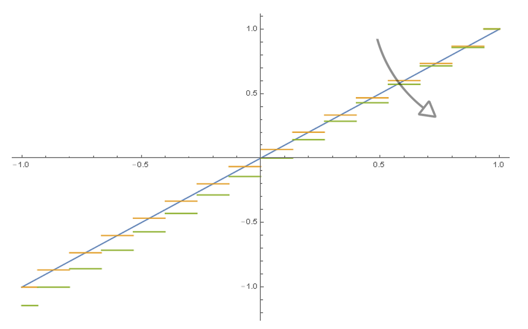
So, to get rid of the quantization error in zero, we have increased the errors, especially for negative numbers. Let’s compare the errors of the two unpacking functions:
$$MeanError(N_{a})=0 \space, \space \space MSE(N_{a})=\frac{1}{3\cdot255^2}$$
$$MeanError(N_{b})=\frac{1}{254} \space, \space \space MSE(N_{b})\approx \frac{1.68}{255^2}$$
Conclusion
So, which unpacking formula is the best, (1) or (2)? We have seen that (1) has a low quantization error but a perturbation of 0.3 degrees for neutral normals. If we use (2) we remove the errors on neutral normals but we increase the general quantization error. It is impossible to get rid of the quantization error, we can only move it and there is no best function. Moreover, since generally a texture map is stored in a compressed format, compression errors are added to quantization errors.
If you want to do manual unpacking using an engine, you should take into account how your engine is storing normal textures. For example, when Unity imports a normal map, it will put the R and G channels of the source file into the G and A channels of the internal texture, thus discarding data in B and A[c]. This because G and A are the two channels that suffer the least from compression and, being the length of a normal vector equal to one and the Z coordinate always positive, we can store only the X and Y coordinates and restore the Z later using the formula:
$$z=\sqrt{1-x^2-y^2}$$
Live Example
 In the sandbox below you can see the two unpacking formulas in action. I’m using a normal map texture with some circles over a neutral layer of color [128, 128, 255]. By toggling the Zero Correction checkbox you can switch between (1) and (2) unpacking formulas. If you pay a very close attention to the neutral zones of the surface and you have a very good screen, you can see a small lighting difference between the two formulas, but it’s barely noticeable.
Notes
- All the vector formulas in this article are component-wise compact functions: each component of the input vector must be evaluated to get the corresponding component of the output vector [↩]
- Low poly as a relative term [↩]
- Unity Normal Map compression [↩]